Categories
pyspark

Transformation and action in pyspark

In this post, let us learn about transformation and action in pyspark.

Transformation

Transformation is one of the operations available in pyspark.

This helps in creating a new RDD from the existing RDD.

Types of transformation

Narrow transformation :

map,filter,flatmap,distinct,sample,union,intersection,join,coalesce,repartition,pipe,cartesian

Wide transformation :

groupByKey,reduceByKey,aggregateByKey,sortByKey

What is action ?

On applying the transformation, DAG(Directed Acyclic Graph)  is usually created. And this develops on further application of some other operations.

But the operations will execute only if action is called upon.

Types of action

reduce,collect,take,head,count,first,saveAsObjectFile,countByKey,foreach,saveAsSequenceFile,saveAsTextFile,takeOrdered,takeSample

Sample program

The following program helps us to filter elements based on some conditions.

But the steps execute only at the collect function. 

from pyspark.sql import SparkSession
from pyspark import SparkContext
sc = SparkContext()
spark = SparkSession(sc)
rdd1=sc.parallelize([1,2,3,4])
rdd1_first=rdd1.filter(lambda x : x<3)
rdd1_first.collect()
[1, 2]

https://beginnersbug.com/rank-and-dense-rank-in-pyspark-dataframe/

https://beginnersbug.com/window-function-in-pyspark-with-example/

Categories
pyspark

Difference between map and flatmap in pyspark

In this post, let us learn about the difference between map and flatmap in pyspark.

What is the difference between Map and Flatmap?

Map and Flatmap are the transformation operations available in pyspark.

The map takes one input element from the RDD and results with one output element. The number of input elements will be equal to the number of output elements.

In the case of Flatmap transformation, the number of elements will not be equal. That is the difference between the two.

Let the below example clarify it clearly.

How to create an RDD ?

With the below part of the code, an RDD is created using parallelize method and its value is viewed.

Let us discuss the topic below with the created RDD.

# Creating RDD using parallelize method
rdd1=sc.parallelize([1,2,3,4])
rdd1.collect()

The RDD contains the following 4 elements.

[1, 2, 3, 4]
How to apply map transformation ?
# Applying map transformation
rdd1_map=rdd1.map(lambda x : x**2)
# Viewing the result
rdd1_map.collect()

In the below result , the output elements are the square of the input elements. And also the count is equal.

[1, 4, 9, 16]
How to apply flatMap transformation ?
# Applying flatmap transformation
rdd1_second=rdd1.flatMap(lambda x : (x**1,x**2))
# Viewing the result
rdd1_second.collect()

In the below result, we are not finding an equal number of elements as map transformation.

[1, 1, 2, 4, 3, 9, 4, 16]

https://beginnersbug.com/transformation-and-action-in-pyspark/

https://beginnersbug.com/spark-sql-operation-in-pyspark/

Categories
pyspark

Subtracting dataframes in pyspark

In this post , let us learn about Subtracting dataframes in pyspark.

Creating dataframes in pyspark

We can create two dataframes using the below program for further use.

Sample program
from pyspark.sql import SparkSession
from pyspark import SparkContext
sc = SparkContext()
spark = SparkSession(sc)
from pyspark.sql import Row<br># Creating the first dataframe df
df=sc.parallelize([Row(name='Gokul',Class=10,level1=480,level2=380,level3=280,level4=520,grade='A'),Row(name='Usha',Class=12,level1=670,level2=720,level3=870,level4=920,grade='A'),Row(name='Rajesh',Class=12,level1=180,level2=560,level3=660,level4=850,grade='B')]).toDF()
print("Printing the dataframe df below")
df.show()<br># Creating the second dataframe df1
df1=sc.parallelize([Row(name='Usha',Class=12,level1=670,level2=720,level3=870,level4=920,grade='A'),Row(name='Kumar',Class=9,level1=320,level2=650,level3=760,level4=580,grade='C')]).toDF()
print("Printing the dataframe df1 below")
df1.show()
Output
Printing the dataframe df below
+-----+-----+------+------+------+------+------+
|Class|grade|level1|level2|level3|level4|  name|
+-----+-----+------+------+------+------+------+
|   10|    A|   480|   380|   280|   520| Gokul|
|   12|    A|   670|   720|   870|   920|  Usha|
|   12|    B|   180|   560|   660|   850|Rajesh|
+-----+-----+------+------+------+------+------+
Printing the dataframe df1 below
+-----+-----+------+------+------+------+-----+
|Class|grade|level1|level2|level3|level4| name|
+-----+-----+------+------+------+------+-----+
|   12|    A|   670|   720|   870|   920| Usha|
|    9|    C|   320|   650|   760|   580|Kumar|
+-----+-----+------+------+------+------+-----+
Subtracting dataframes

The keyword subtract helps us in subtracting dataframes in pyspark.

In the below program, the first dataframe is subtracted with the second dataframe.

#Subtracting dataframes in pyspark
df2=df.subtract(df1)
print("Printing the dataframe df2 below")
df2.show()
Printing the dataframe df2 below
+-----+-----+------+------+------+------+------+
|Class|grade|level1|level2|level3|level4|  name|
+-----+-----+------+------+------+------+------+
|   10|    A|   480|   380|   280|   520| Gokul|
|   12|    B|   180|   560|   660|   850|Rajesh|
+-----+-----+------+------+------+------+------+

We can subtract the dataframes based on few columns also.

#Subtracting dataframes based on few columns
df3=df.select('Class','grade','level1').subtract(df1.select('Class','grade','level1'))
print("Printing the dataframe df3 below ")
df3.show()
Printing the dataframe df3 below
+-----+-----+------+
|Class|grade|level1|
+-----+-----+------+
|   10|    A|   480|
|   12|    B|   180|
+-----+-----+------+
Reference

http://spark.apache.org/docs/latest/api/python/pyspark.html?highlight=subtract#pyspark.RDD.subtract

Categories
pyspark

greatest() and least() in pyspark

In this post, we will learn the functions greatest() and least() in pyspark.

greatest() in pyspark

Both the functions greatest() and least() helps in identifying the greater and smaller value among few of the columns.

Creating dataframe

With the below sample program, a dataframe can be created which could be used in the further part of the program.

To understand the creation of dataframe better, please refer to the earlier post

Sample program
from pyspark.sql import SparkSession
from pyspark import SparkContext
sc = SparkContext()
spark = SparkSession(sc)
from pyspark.sql import Row
df=sc.parallelize([Row(name='Gokul',Class=10,level1=480,level2=380,level3=280,level4=520,grade='A'),Row(name='Usha',Class=12,level1=670,level2=720,level3=870,level4=920,grade='A'),Row(name='Rajesh',Class=12,level1=180,level2=560,level3=660,level4=850,grade='B')]).toDF()
print("Printing the dataframe df below")
Output
Printing the dataframe df below
+-----+-----+------+------+------+------+------+
|Class|grade|level1|level2|level3|level4|  name|
+-----+-----+------+------+------+------+------+
|   10|    A|   480|   380|   280|   520| Gokul|
|   12|    A|   670|   720|   870|   920|  Usha|
|   12|    B|   180|   560|   660|   850|Rajesh|
+-----+-----+------+------+------+------+------+
greatest() in pyspark

In order to compare the multiple columns row-wise, the greatest and least function can be used.

In the below program, the four columns level1,level2,level3,level4 are getting compared to find the larger value.

Sample program
from pyspark.sql.functions import greatest,col
df1=df.withColumn("large",greatest(col("level1"),col("level2"),col("level3"),col("level4")))
print("Printing the dataframe df1 below")
df1.show()

The column large is populated with the greater value among the four levels for each row .

Output
Printing the dataframe df1 below
+-----+-----+------+------+------+------+------+-----+
|Class|grade|level1|level2|level3|level4|  name|large|
+-----+-----+------+------+------+------+------+-----+
|   10|    A|   480|   380|   280|   520| Gokul|  520|
|   12|    A|   670|   720|   870|   920|  Usha|  920|
|   12|    B|   180|   560|   660|   850|Rajesh|  850|
+-----+-----+------+------+------+------+------+-----+
least() in pyspark

The least function helps us to get a smaller value among the four levels for each row. 

Sample program
from pyspark.sql.functions import least,col
df2=df.withColumn("Small",least(col("level1"),col("level2"),col("level3"),col("level4")))
print("Printing the dataframe df2 below")
df2.show()
Output
Printing the dataframe df2 below
+-----+-----+------+------+------+------+------+-----+
|Class|grade|level1|level2|level3|level4|  name|Small|
+-----+-----+------+------+------+------+------+-----+
|   10|    A|   480|   380|   280|   520| Gokul|  280|
|   12|    A|   670|   720|   870|   920|  Usha|  670|
|   12|    B|   180|   560|   660|   850|Rajesh|  180|
+-----+-----+------+------+------+------+------+-----+
Reference

https://spark.apache.org/docs/2.1.0/api/python/pyspark.sql.html#pyspark.sql.functions.greatest

https://spark.apache.org/docs/2.1.0/api/python/pyspark.sql.html#pyspark.sql.functions.least

Categories
pyspark

spark SQL operation in pyspark

In this post, let us look into the spark SQL operation in pyspark with example.

What is spark SQL in pyspark ?

Spark SQL helps us to execute SQL queries. We can store a dataframe as table using the function createOrReplaceTempView.

Sample program

In the following sample program, we are creating an RDD using parallelize method and later converting it into dataframe.

To understand the process of creating dataframes better, Please refer to the below link.

createOrReplaceTempView helps us to register the dataframe created as temporary table.

We can execute all the SQL queries with the help of spark SQL operation in pyspark.

#Libraries required
from pyspark.sql import SparkSession
from pyspark import SparkContext
sc = SparkContext()
spark = SparkSession(sc)
from pyspark.sql import Row
#creating rdd and converting to dataframe
df=sc.parallelize([Row(name='Gokul',Class=10,marks=480,grade='A'),Row(name='Usha',Class=12,marks=450,grade='A'),Row(name='Rajesh',Class=12,marks=430,grade='B')]).toDF()
#Registering temporary table with create dataframedf.createOrReplaceTempView("df_view")
#Executing SQl queries using spark SQl operation
spark.sql("select * from df_view").show()
Output

We can even manipulate the data by filtering based on some conditions using where clause.

But Below is the entire data of the dataframe without any filteration and modification.

+-----+-----+-----+------+
|Class|grade|marks|  name|
+-----+-----+-----+------+
|   10|    A|  480| Gokul|
|   12|    A|  450|  Usha|
|   12|    B|  430|Rajesh|
+-----+-----+-----+------+
Reference

https://stackoverflow.com/questions/32788387/pipelinedrdd-object-has-no-attribute-todf-in-pyspark

Categories
pyspark

rank and dense rank in pyspark dataframe

In this post, Let us know rank and dense rank in pyspark dataframe using window function with examples.

Rank and dense rank

The rank and dense rank in pyspark dataframe help us to rank the records based on a particular column.

This works in a similar manner as the row number function .To understand the row number function in better, please refer below link.

The row number function will work well on the columns having non-unique values . Whereas rank and dense rank help us to deal with the unique values.

Sample program – creating dataframe

We could create the dataframe containing the salary details of some employees from different departments using the below program.

from pyspark.sql import Row
# Creating dictionary with employee and their salary details 
dict1=[{"Emp_id" : 123 , "Dep_name" : "Computer"  , "Salary" : 2500 } , {"Emp_id" : 456 ,"Dep_name"  :"Economy" , "Salary" : 4500} , {"Emp_id" : 789 , "Dep_name" : "Economy" , "Salary" : 7200 } , {"Emp_id" : 564 , "Dep_name" : "Computer" , "Salary" : 1400 } , {"Emp_id" : 987 , "Dep_name" : "History" , "Salary" : 3450 }, {"Emp_id" :678 , "Dep_name" :"Economy" ,"Salary": 4500},{"Emp_id" : 943 , "Dep_name" : "Computer" , "Salary" : 3200 }]
# Creating RDD from the dictionary created above
rdd1=sc.parallelize(dict1)
# Converting RDD to dataframe
df1=rdd1.toDF()
print("Printing the dataframe df1")
df1.show()
Printing the dataframe df1
+--------+------+------+
|Dep_name|Emp_id|Salary|
+--------+------+------+
|Computer|   123|  2500|
| Economy|   456|  4500|
| Economy|   789|  7200|
|Computer|   564|  1400|
| History|   987|  3450|
| Economy|   678|  4500|
|Computer|   943|  3200|
+--------+------+------+
Sample program – rank()

In order to use the rank and dense rank in our program, we require below libraries.

from pyspark.sql import Window
from pyspark.sql.functions import rank,dense_rank

from pyspark.sql import Window
from pyspark.sql.functions import rank
df2=df1.withColumn("rank",rank().over(Window.partitionBy("Dep_name").orderBy("Salary")))
print("Printing the dataframe df2")
df2.show()

In the below output, the department economy contains two employees with the first rank. This is because of the same salary being provided for both employees.

But instead of assigning the next salary with the second rank, it is assigned with the third rank. This is how the rank function will work by skipping the ranking order.

Printing the dataframe df2
+--------+------+------+----+
|Dep_name|Emp_id|Salary|rank|
+--------+------+------+----+
|Computer|   564|  1400|   1|
|Computer|   123|  2500|   2|
|Computer|   943|  3200|   3|
| History|   987|  3450|   1|
| Economy|   456|  4500|   1|
| Economy|   678|  4500|   1|
| Economy|   789|  7200|   3|
+--------+------+------+----+
Sample program – dense rank()

In the dense rank, we can skip the ranking order . For the same scenario discussed earlier, the second rank is assigned in this case instead of skipping the sequence order. 

from pyspark.sql import Window
from pyspark.sql.functions import dense_rank
df3=df1.withColumn("denserank",dense_rank().over(Window.partitionBy("Dep_name").orderBy("Salary")))
print("Printing the dataframe df3")
df3.show()
Printing the dataframe df3
+--------+------+------+---------+
|Dep_name|Emp_id|Salary|denserank|
+--------+------+------+---------+
|Computer|   564|  1400|        1|
|Computer|   123|  2500|        2|
|Computer|   943|  3200|        3|
| History|   987|  3450|        1|
| Economy|   456|  4500|        1|
| Economy|   678|  4500|        1|
| Economy|   789|  7200|        2|
+--------+------+------+---------+
Reference

http://spark.apache.org/docs/latest/api/python/pyspark.sql.html?highlight=window#pyspark.sql.Column.over

Categories
pyspark

row_number in pyspark dataframe

In this post, we will learn to use row_number in pyspark dataframe with examples.

What is row_number ?

This row_number in pyspark dataframe will assign consecutive numbering over a set of rows.
The window function in pyspark dataframe helps us to achieve it.
To get to know more about window function, Please refer to the below link.

Creating dataframe 

Before moving into the concept, Let us create a dataframe using the below program.

from pyspark.sql import Row
# Creating dictionary with employee and their salary details 
dict1=[{"Emp_id" : 123 , "Dep_name" : "Computer"  , "Salary" : 2500 } , {"Emp_id" : 456 ,"Dep_name"  :"Economy" , "Salary" : 4500} , {"Emp_id" : 789 , "Dep_name" : "Economy" , "Salary" : 7200 } , {"Emp_id" : 564 , "Dep_name" : "Computer" , "Salary" : 1400 } , {"Emp_id" : 987 , "Dep_name" : "History" , "Salary" : 3450 }, {"Emp_id" :678 , "Dep_name" :"Economy" ,"Salary": 6700},{"Emp_id" : 943 , "Dep_name" : "Computer" , "Salary" : 3200 }]
# Creating RDD from the dictionary created above
rdd1=sc.parallelize(dict1)
# Converting RDD to dataframe
df1=rdd1.toDF()
print("Printing the dataframe df1")
df1.show()

Thus we created the below dataframe with the salary details of some employees from various departments.

Printing the dataframe df1
+--------+------+------+
|Dep_name|Emp_id|Salary|
+--------+------+------+
|Computer|   123|  2500|
| Economy|   456|  4500|
| Economy|   789|  7200|
|Computer|   564|  1400|
| History|   987|  3450|
| Economy|   678|  6700|
|Computer|   943|  3200|
+--------+------+------+
Sample program – row_number

With the below segment of the code, we can populate the row number based on the Salary for each department separately.

We need to import the following libraries before using the window and row_number in the code.

orderBy clause is used for sorting the values before generating the row number.

from pyspark.sql import Window
from pyspark.sql.functions import row_number
df2=df1.withColumn("row_num",row_number().over(Window.partitionBy("Dep_name").orderBy("Salary")))
print("Printing the dataframe df2")
df2.show()
Printing the dataframe df2
+--------+------+------+-------+
|Dep_name|Emp_id|Salary|row_num|
+--------+------+------+-------+
|Computer|   564|  1400|      1|
|Computer|   123|  2500|      2|
|Computer|   943|  3200|      3|
| History|   987|  3450|      1|
| Economy|   456|  4500|      1|
| Economy|   678|  6700|      2|
| Economy|   789|  7200|      3|
+--------+------+------+-------+
Reference

https://spark.apache.org/docs/2.1.0/api/python/pyspark.sql.html#pyspark.sql.functions.row_number

Categories
pyspark

window function in pyspark with example

In this post, We will learn about window function in pyspark with example.

What is window function ?

Window function in pyspark acts in a similar way as a group by clause in SQL.

It basically groups a set of rows based on the particular column and performs some aggregating function over the group.

Sample program for creating dataframe

For understanding the concept better, we will create a dataframe containing the salary details of some employees using the below program.

# Creating dictionary with employee and their salary details 
dict1=[{"Emp_id" : 123 , "Dep_name" : "Computer"  , "Salary" : 2500 } , {"Emp_id" : 456 ,"Dep_name"  :"Economy" , "Salary" : 4500} , {"Emp_id" : 789 , "Dep_name" : "History" , "Salary" : 6700 } , {"Emp_id" : 564 , "Dep_name" : "Computer" , "Salary" : 1400 } , {"Emp_id" : 987 , "Dep_name" : "History" , "Salary" : 3450 }, {"Emp_id" :678 , "Dep_name" :"Economy" ,"Salary": 6700}]
# Creating RDD from the dictionary created above
rdd1=sc.parallelize(dict1)
# Converting RDD to dataframe
df1=rdd1.toDF()
print("Printing the dataframe df1")
df1.show()
Printing the dataframe df1
+--------+------+------+
|Dep_name|Emp_id|Salary|
+--------+------+------+
|Computer|   123|  2500|
| Economy|   456|  4500|
| History|   789|  6700|
|Computer|   564|  1400|
| History|   987|  3450|
| Economy|   678|  6700|
+--------+------+------+
How to use window function in our program?

In the below segment of code, the window function used to get the sum of the salaries over each department.

The following library is required before executing the code.

from pyspark.sql import Window

partitionBy includes the column name based on which the grouping needs to be done.

df = df1.withColumn("Sum",sum('Salary').over(Window.partitionBy('Dep_name')))
print("Printing the result")
df.show()
Printing the result
+--------+------+------+-----+
|Dep_name|Emp_id|Salary|  Sum|
+--------+------+------+-----+
|Computer|   123|  2500| 3900|
|Computer|   564|  1400| 3900|
| History|   789|  6700|10150|
| History|   987|  3450|10150|
| Economy|   456|  4500|11200|
| Economy|   678|  6700|11200|
+--------+------+------+-----+
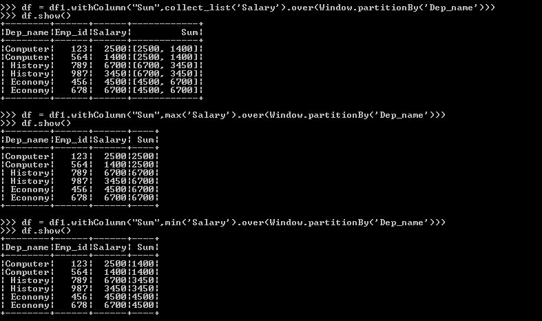
Other aggregate functions

As above, we can do for all the other aggregate functions also. Some of those aggregate functions are max(),Avg(),min(),collect_list().

Below are the few examples of those aggregate functions.

window function with some other aggregate functions

Reference

https://medium.com/@rbahaguejr/window-function-on-pyspark-17cc774b833a

Window function in pyspark with example using advanced aggregate functions like row_number(), rank(),dense_rank() can be discussed in our other blogs .

Categories
pyspark

Left-anti and Left-semi join in pyspark

In this post, We will learn about Left-anti and Left-semi join in pyspark dataframe with examples.

Sample program for creating dataframes

Let us start with the creation of two dataframes . After that we will move into the concept of Left-anti and Left-semi join in pyspark dataframe.

# Creating two dictionaries with Employee and Department details
dict=[{"Emp_id" : 123 , "Emp_name" : "Raja" },{"Emp_id" : 234 , "Emp_name" : "Sindu"},{"Emp_id" : 456 , "Emp_name" : "Ravi"}]
dict1=[{"Emp_id" : 123 , "Dep_name" : "Computer" } , {"Emp_id" : 456 ,"Dep_name"  :"Economy"} , {"Emp_id" : 789 , "Dep_name" : "History"}]
# Creating RDDs from the above dictionaries using parallelize method
rdd=sc.parallelize(dict)
rdd1=sc.parallelize(dict1)
# Converting RDDs to dataframes 
df=rdd.toDF()
df1=rdd1.toDF()
print("Printing the first dataframe")
df.show()
print("Printing the second dataframe")
df1.show()
Printing the first dataframe
+------+--------+
|Emp_id|Emp_name|
+------+--------+
|   123|    Raja|
|   234|   Sindu|
|   456|    Ravi|
+------+--------+
Printing the second dataframe
+--------+------+
|Dep_name|Emp_id|
+--------+------+
|Computer|   123|
| Economy|   456|
| History|   789|
+--------+------+
What is Left-anti join ?

In order to return only the records available in the left dataframe . For those does not have the matching records in the right dataframe, We can use this join.

We could even see in the below sample program . Only the columns from the left dataframe will be available in Left-anti and Left-semi . And not all  the columns from both the dataframes as in other types of joins.

Sample program – Left-anti join

Emp_id: 234 is only available in the left dataframe and not in the right dataframe.

# Left-anti join between the two dataframes df and df1 based on the column Emp_id
df2=df.join(df1,['Emp_id'], how = 'left_anti')
print("Printing the result of left-anti below")
df2.show()
Printing the result of left-anti below
+------+--------+
|Emp_id|Emp_name|
+------+--------+
|   234|   Sindu|
+------+--------+
What is Left-semi join?

The common factors between the two dataframes is listed down in this join.

In the below sample program, two Emp_ids -123,456 are available in both the dataframes and so they picked up here.

Sample program – Left-semi join
# Left-semi join between two dataframes df and df1
df3=df.join(df1,['Emp_id'], how = 'left_semi')
print("Printing the result of left-semi below")
df3.show()
Printing the result of left-semi below
+------+--------+
|Emp_id|Emp_name|
+------+--------+
|   123|    Raja|
|   456|    Ravi|
+------+--------+

Other types of join are outer join  and inner join in pyspark 

Reference

https://spark.apache.org/docs/latest/api/python/pyspark.sql.html?highlight=join#pyspark.sql.DataFrame.join

Categories
pyspark

Outer join in pyspark dataframe with example

In this post , we will learn about outer join in pyspark dataframe with example .

If you want to learn Inner join refer below URL

There are other types of joins like inner join , left-anti join and left semi join

What you will learn

At the end of this tutorial, you will learn Outer join in pyspark dataframe with example

Types of outer join

Types of outer join in pyspark dataframe are as follows :

  • Right outer join / Right join 
  • Left outer join / Left join
  • Full outer join /Outer join / Full join 
Sample program for creating two dataframes

We will start with the creation of two dataframes before moving into the topic of outer join in pyspark dataframe .

#Creating dictionaries
dict=[{"Emp_id" : 123 , "Emp_name" : "Raja" },{"Emp_id" : 234 , "Emp_name" : "Sindu"},{"Emp_id" : 456 , "Emp_name" : "Ravi"}]
dict1=[{"Emp_id" : 123 , "Dep_name" : "Computer" } , {"Emp_id" : 456 ,"Dep_name"  :"Economy"} , {"Emp_id" : 789 , "Dep_name" : "History"}]
# Creating RDDs from the above dictionaries using parallelize method
rdd=sc.parallelize(dict)
rdd1=sc.parallelize(dict1)
# Converting RDDs to dataframes 
df=rdd.toDF()
df1=rdd1.toDF()
print("Printing the first dataframe")
df.show()
print("Printing the second dataframe")
df1.show()
Printing the first dataframe
+------+--------+
|Emp_id|Emp_name|
+------+--------+
|   123|    Raja|
|   234|   Sindu|
|   456|    Ravi|
+------+--------+
Printing the second dataframe
+--------+------+
|Dep_name|Emp_id|
+--------+------+
|Computer|   123|
| Economy|   456|
| History|   789|
+--------+------+
What is Right outer join ?

The Right outer join helps us to get the entire records from the right dataframe along with the matching records from the left dataframe .

And will be populated with null for the remaining unmatched columns of the left dataframe.

Sample program – Right outer join / Right join

Within the join syntax , the type of join to be performed will be mentioned as right_outer or right .

As Emp_name for Emp_id : 789 is not available in the left dataframe , it is populated with null in the following result .

# Right outer join / Right join 
df2=df.join(df1,['Emp_id'], how = 'right_outer')
print("Printing the result of right outer / right join")
df2.show()
# Printing the result of right outer / right join 
+------+--------+--------+
|Emp_id|Emp_name|Dep_name|
+------+--------+--------+
|   789|    null| History|
|   123|    Raja|Computer|
|   456|    Ravi| Economy|
+------+--------+--------+
What is Left outer join ?

This join is used to retrieve all the records from the left dataframe with its matching records from right dataframe .

The type of join is mentioned in either way as Left outer join or left join .

Sample program – Left outer join / Left join

In the below example , For the Emp_id : 234 , Dep_name is populated with null as there is no record for this Emp_id in the right dataframe .

# Left outer join / Left join <br />df3=df.join(df1,['Emp_id'], how = 'left_outer')
Print("Printing the result of Left outer join / Left join") 
 df3.show()
Printing the result of Left outer join / Left join
+------+--------+--------+
|Emp_id|Emp_name|Dep_name|
+------+--------+--------+
|   234|   Sindu|    null|
|   123|    Raja|Computer|
|   456|    Ravi| Economy|
+------+--------+--------+
What is Full outer join ?

Full outer join generate the result with all the records from both the dataframes . Null will populate in the columns for the unmatched records  .

Sample program – Full outer join / Full join / Outer join

All the Emp_ids from both the dataframes combined in this case with null population for unavailable values .

# Full outer join / Full join / Outer join
df4=df.join(df1,['Emp_id'], how = 'Full_outer')
print(Printing the result of Full outer join")
df4.show()
Printing the result of Full outer join
+------+--------+--------+
|Emp_id|Emp_name|Dep_name|
+------+--------+--------+
|   789|    null| History|
|   234|   Sindu|    null|
|   123|    Raja|Computer|
|   456|    Ravi| Economy|
+------+--------+--------+
Reference

https://spark.apache.org/docs/latest/api/python/reference/api/pyspark.sql.DataFrame.join.html?highlight=outer%20join